Using the Red Pitaya STEMlab 125-14 PRO Gen2 as an SDR in GNU Radio
The Red Pitaya STEMlab 125-14 PRO Gen2 slogan is “The swiss army knife for engineers”, and it is very true. The board is a compact Zynq-based system with two analog inputs and two analog outputs, and it can be used as a signal generator, an oscilloscope, a spectrum analyzer, a logic analyzer, a function generator, and essentially any other applications about reading a signal or generating a signal or both together. Then we have a set of software applications that run on the board and give you a web interface to read and generate signals. In this blog we already covered the Red Pitaya STEMlab as a spectrum analyzer in a previous article using the built-in web applications. Also, we used it from a Python application running in a host computer, and using SCPI commands to control the board.
This time we are going to use another different interface: the Red Pitaya as a software-defined radio inside GNU Radio, where the STEMlab becomes the digitizer and all the signal processing lives in a flowgraph on my computer.
Table of contents
- The Red Pitaya blocks for GNU Radio
- Preparing the board to accept connections
- A first experiment: filtering a signal
- Why GNU Radio is not made for this
- From a signal generator to an antenna
- Receiving 94.2 MHz with a 125 MSPS ADC
- The analog wall
- Conclusions
The Red Pitaya blocks for GNU Radio
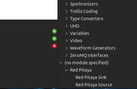
The Red Pitaya source and sink blocks for GNU Radio come from Pavel Demin’s red-pitaya-notes repository. They live inside the SDR transceiver project:
git clone https://github.com/pavel-demin/red-pitaya-notes.git
cd red-pitaya-notes/projects/sdr_transceiver/gnuradio
From this repository, I’ve created a repository on my GitHub named redpitaya_projects that contains the same blocks plus a few flowgraphs I used to test them. The repository also includes the import_blocks.sh script that sets the environment variables GNU Radio needs to find the blocks and launches GNU Radio Companion (GRC).
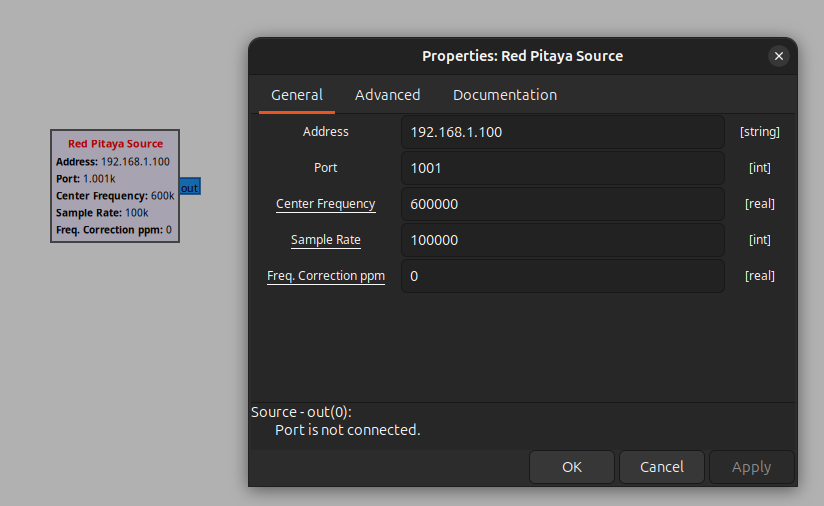
In the original repository, we can find two GNU Radio blocks: a source, which makes the Red Pitaya read a signal from one of its ADC channels and stream it to the host, and a sink, which makes the board generate a signal through one of its DAC channels.
What is worth understanding before drawing any flowgraph is how these blocks are built, because it explains every limitation later in this article. The implementation has two halves. On the board there is an HTTP server together with a set of HDL modules that configure the DACs and ADCs and implement a digital down-converter (DDC) in the FPGA fabric. On the host there are a couple of XML files that define the GRC blocks plus a Python script, red_pitaya.py, that opens TCP sockets to the board and sends the configuration commands.
This is the key point: the GNU Radio block is essentially a gr.hier_block2 wrapping two sockets. A control socket carries the tuning frequency and the sample rate, and a data socket carries a stream of complex gr_complex samples read straight from a file_descriptor_source. Nothing you draw in your flowgraph runs on the Red Pitaya. The board acquires, decimates, and ships samples; every block you add afterwards executes on your computer. (This is not valid only for this board, is the way most SDR front-ends work, including the USRP and the HackRF).
The source block exposes the parameters you would expect from an SDR front-end: the board address and port, the center frequency, the sample rate, and a frequency correction in ppm.
Preparing the board to accept connections
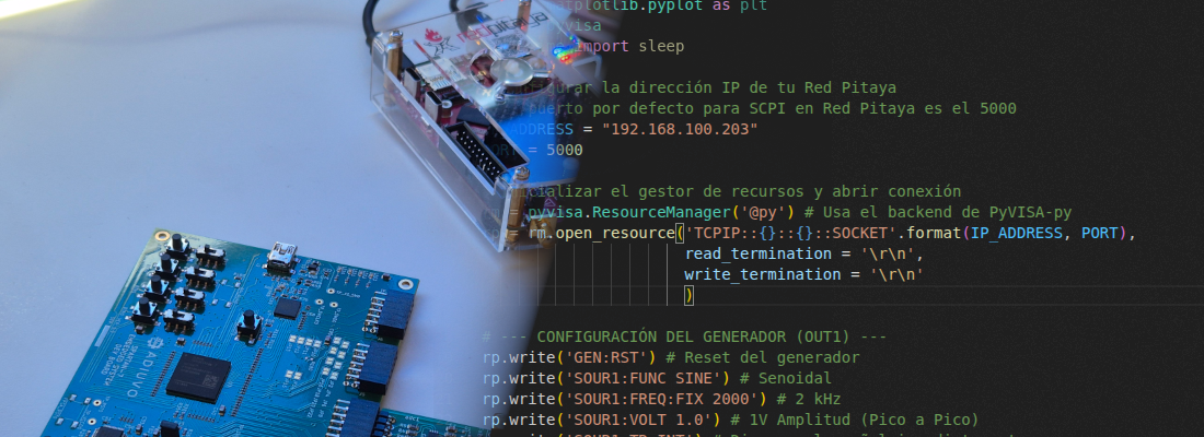
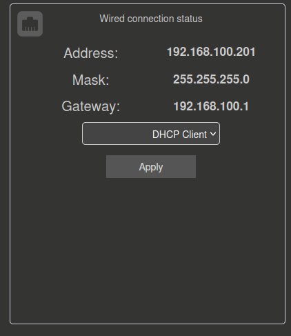
Before GNU Radio can talk to the board, two things need to be in place. First, you need the Red Pitaya’s IP address. You can navigate to the Red Pitaya Network Manager in the web interface and read it there. In my setup the board sits at 192.168.100.201.
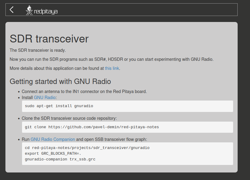
Second, and this is easy to forget, you need to launch the SDR transceiver application from the Red Pitaya home page. That application is the server side of the pavel-demin blocks, and until it is running the board will simply not answer the sockets. If you only boot the stock image and never open that app, the source block streams nothing useful and you stare at a flat noise floor wondering why.
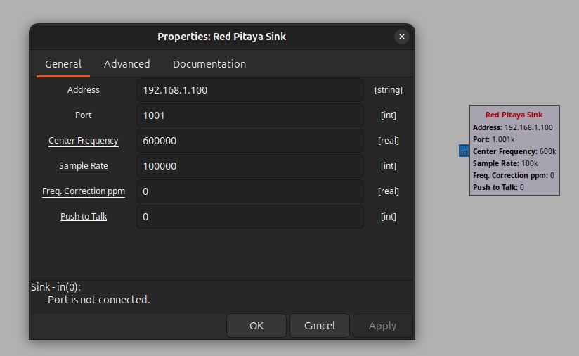
The port number selects the channel. Configuring the block to port 1001 works with channel 1, while port 1002 works with channel 2, so the same flowgraph can address either analog front-end just by changing the port. The sink block is almost identical to the source, with one extra parameter: a Push to talk field that must be set to True to actually enable the output channel.
A first experiment: filtering a signal
My first idea was naive but instructive: use the Red Pitaya as a real-time DSP engine. Read a signal with the source, run it through a GNU Radio filter, and play it back out through the sink. A hardware-in-the-loop filter, basically.
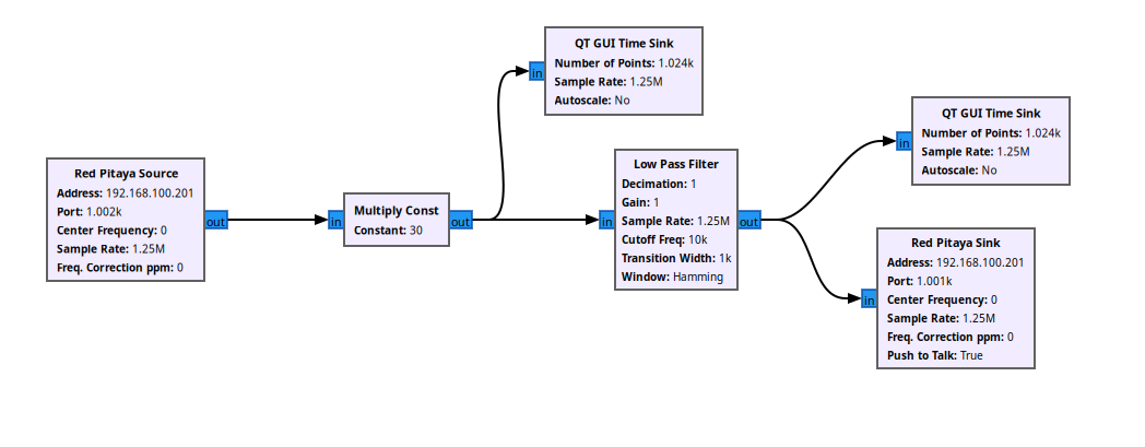
The flowgraph is simple. The source is tuned with its center frequency set to 0, the sample rate is set through a variable to 1.25 MSPS, and the IP address is another variable pointing at 192.168.100.201. After the source I added a low-pass filter and routed the result to the sink. There are two details that already tell you something is off.
The first is that I had to insert a Multiply Const block right after the source. The samples that come out of the Red Pitaya source are not volts; they are normalized values around full scale, so without a gain block the numbers are meaningless as a physical measurement. The exact factor depends on the analog jumper (LV gives ±1 V, HV gives ±20 V) and on the DDC gain, so it has to be calibrated empirically against a known input.
The second detail is that the center frequency has to be 0, which means that we are going to capture a baseband signal.
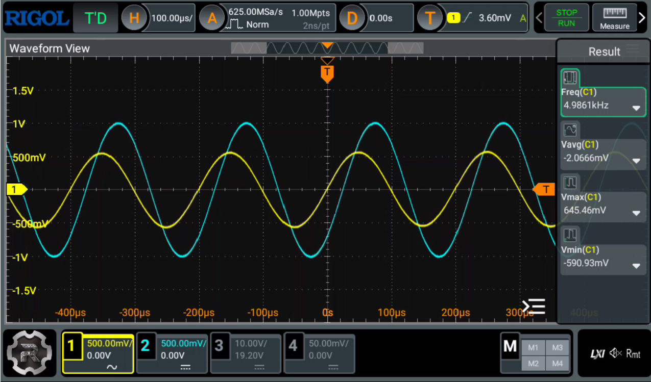
With a function generator feeding a 5 kHz sine into the input, the filtered output appears, We can see a shift between the input and the output signals, however this is not because of the delay added by the DSP chain, but because the tipical delay of the FIR filter, at least the most of it.
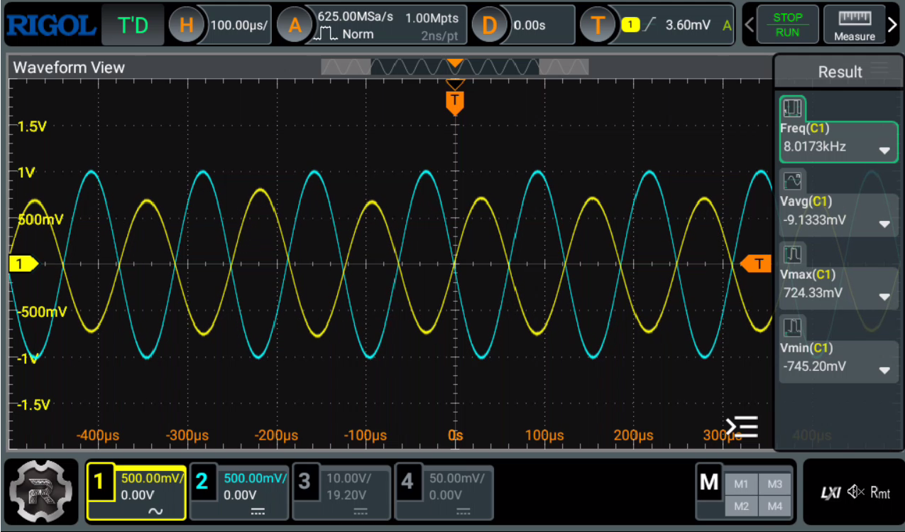
Pushing the generator to 8 kHz, we can see that the delay changes. I checked that this delay is linear with the frequency, so it is an expected behavior of the filter. However, in reality, we would need to make more tests in order to extract which is the exact delay of the filter, and the delay of the DSP chain.
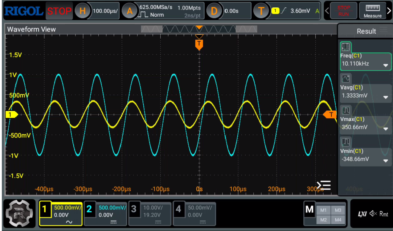
Finally feeding a tone above the 10 kHz cutoff of the filter, the output is attenuated as expected.
Why GNU Radio is not made for this
That changing phase between 5 kHz and 8 kHz is worth a paragraph, because it confused me at first and the explanation is pure DSP. The low-pass filter in GNU Radio is a linear-phase FIR, which means it has a constant group delay: every frequency in the passband is delayed by exactly the same amount of time, (N-1)/2 samples. A constant time delay does not look like a constant phase, though. The phase it produces grows linearly with frequency, φ = -2π·f·τ, so a fixed delay shows up as one angle at 5 kHz and a completely different angle at 8 kHz.
On top of that constant filter delay sits the real problem: the samples make a round trip across the network to the host and back, and that adds a large, uncontrollable latency that has nothing to do with your filter design. The high-speed path inside the Red Pitaya STEMlab is only used to acquire and stream; the processing happens on the host, packaged into TCP, with all the buffering that implies. Again, this is not a problem of this board in particular, but of any SDR front-end connected to GNU Radio.
When I started thinking about this use of the Red Pitaya STEMlab, I assumed I would be able to use the GNU Radio GUI to implement DSP algorithms for ordinary signals. I was wrong, and in hindsight it makes sense. To make even this trivial flowgraph behave I had to add an input gain because the samples are not volts, I had to force the center frequency to zero, and I still ended up with an uncontrollable delay in the output. GNU Radio is simply not built to be a deterministic, low-latency DSP box. It is built for radio. So let’s use it for radio.
From a signal generator to an antenna
The fix is to change the approach entirely: replace the signal generator with an antenna. A fairly long one, because the interesting low-frequency RF lives down in the HF range and a short wire will not couple much energy into it. Once you stop thinking of the STEMlab as a filter and start thinking of it as a receiver front-end, everything the blocks do (tune with the DDC, decimate, stream I/Q) is exactly what you want.
The natural target for a first test is commercial FM broadcast, something strong and easy to find, like a local station at 94.2 MHz. And that is where the fun begins, because a 94.2 MHz signal and a 125 MSPS ADC do not get along in the obvious way.
Receiving 94.2 MHz with a 125 MSPS ADC
The Red Pitaya samples at a maximum of 125 MSPS. According to Nyquist, that means it can represent frequencies only up to 62.5 MHz. A station at 94.2 MHz is well above that limit, so direct sampling is out of the question.
But there is a trick. Sampling at 125 MSPS does not delete energy above Nyquist, it folds it. A signal sitting at 94.2 MHz lives in the second Nyquist zone, and after sampling it also appears at:
\[f_{alias} = |f_{RF} - f_s| = |94.2 - 125| = 30.8 \ \text{MHz}\]So the FM station shows up, aliased, at 30.8 MHz inside the digitized spectrum. This is undersampling, or bandpass sampling, and it is a perfectly legitimate technique. The consequence for the flowgraph is simple: I tune the DDC center frequency not to 94.2 MHz, which the NCO cannot represent anyway, but to 30.8 MHz, where the alias actually lands.
# 94.2 MHz commercial FM, sampled at 125 MSPS, aliases to:
#   |94.2e6 - 125e6| = 30.8 MHz
center_frequency = 30800000
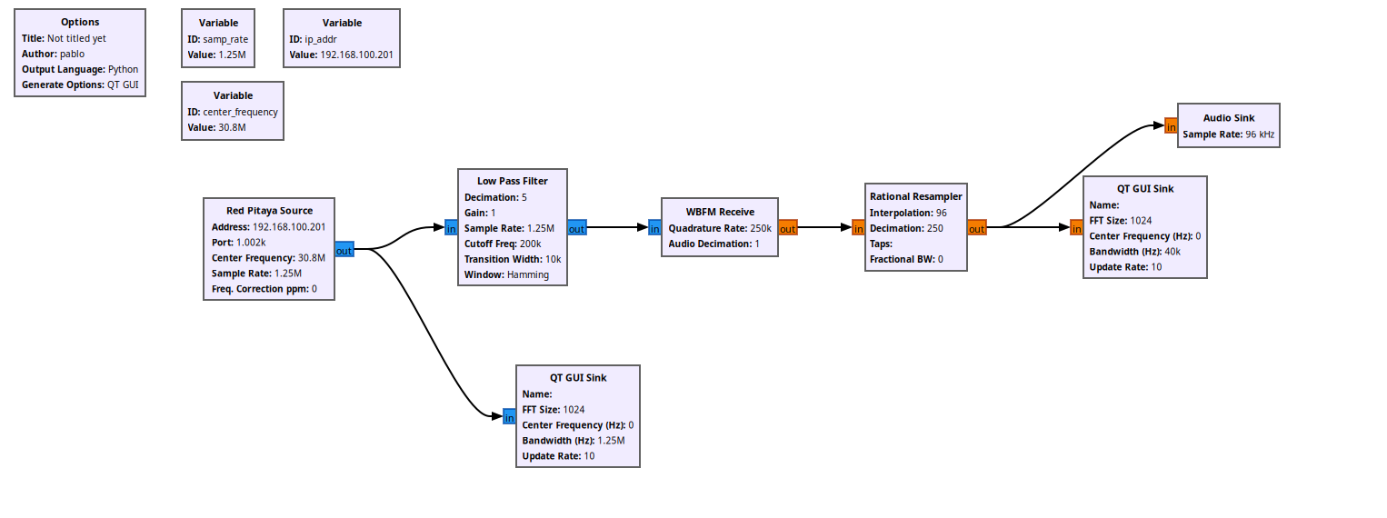
From there the rest is a textbook wideband FM receiver: a channel low-pass filter, a WBFM Receive block fed at a quadrature rate of 250 kSPS, a rational resampler down to a 96 kHz audio rate, and an audio sink. Notice that the second Nyquist zone folds with its spectrum inverted, but for mono FM that inversion is inaudible, so it does not get in the way. For the sake of this test, where I only want to see if the station is there, we can ignore the audio signal.
On paper this should work. The digital side is solved. The problem is on the analog side.
The analog side
When I ran the flowgraph, all I got was white noise. No station, just the noise floor. And this is not a bug in the flowgraph, it is physics.
The analog RF input of the Red Pitaya STEMlab 125-14 is limited to roughly 60 MHz of bandwidth, with an anti-aliasing filter in front of the ADC that is there precisely to stop signals from the second Nyquist zone from folding in. That filter does exactly its job: it attenuates 94.2 MHz so heavily that, even though the alias would land neatly at 30.8 MHz, there is almost nothing left of the signal by the time it reaches the converter. The clever digital trick is real, but the front-end was designed to defeat it.
This is, by the way, the reason the Red Pitaya SDRlab 122-16 exists. Its analog front-end reaches much higher frequencies, so it can genuinely exploit undersampling to receive signals far above its own Nyquist limit. The Red Pitaya STEMlab 125-14 PRO Gen 2 is simply not that board. What it does well, and what it was built for, is receiving anything below ~60 MHz and decoding it without any of these contortions: the HF amateur bands, shortwave broadcast, the AM band, and so on. Tune the DDC to a frequency the front-end actually passes, hang a long enough wire on the input, and the same flowgraph that heard only noise at 94.2 MHz will happily pull in real stations.
Conclusions
The first time I thought of using the Red Pitaya STEMlab as a software-defined radio inside GNU Radio, I imagined it would be a simple way to implement DSP algorithms on real signals, however the architecture of the pavel-demin blocks plus how GNU Radio works makes that impossible for real-time, at least in the way I imagined it.
However, could be interesting to create a set of blocks that run on the PL side of the Zynq and implement DSP algorithms there, so the flowgraph would run on the PL and the Red Pitaya would be a real-time DSP engine. Actually this is very possible because the Red Pitaya team shared an article explaining how to create your own web applications that runs on the Zynq. This could be the topic for a future article.
The code of this article is uploaded to GitHub.