Understanding the PID regulator.
I always remember when the Optimization and Optimum Control teacher at the university told us that 90% of the regulators we will find in our life, will be PID, 5% will be LQR and the other 5% will be other complex regulators. PID control has become the most used control because of its simplicity both in the implementation of them, and in their adjustment, and they can be used even without knowing what it is doing exactly. In this article, we will see that the PID regulator is a filter, and as a filter, they have all the parameters of the filters like natural frequency, cut frequency, or quality factor, configured according to their constants.
The simplest regulator we can implement, is a proportional regulator. This regulator is just a gain applied to the error, and its behavior depends on the gain of the system. The equation of this regulator is the next.
\[H(s)=K\]This kind of regulator can be useful when we don’t need the output to reach exactly the value of the reference, or when the gain of the feedback system is equal to one. In this case, the system will reach the reference. In all the other cases, this regulator is not used.
Since usually we need that the output follow the reference, the most used regulator is the proportional - integral regulator or PI. The equation of this regulator is the next.
\[H(s)=K_p+K_i \cdot \frac{1}{s}\]We can implement this equation on the FPGA and change the values of Kp and Ki to get the desired response of the system, but it is useful to know the response of the regulator to estimate from the beginning values for the regulator constants. To know the response of any system, we can calculate its bode diagram, and obtain the equation of the different parameters of the bode diagram such as natural frequencies of gain. To obtain these parameters we need to operate a little bit the PI equation.
Firstly, we are going to isolate the Kp constant. This makes sense if you think on this constant as a gain of the entire system.
\[H(s)=K_p \left( 1+\frac{\frac{K_i}{K_p}}{s} \right)\]Now we can make the \(s\) variable as a common denominator.
\[H(s)= K_p \left( \frac{s+\frac{K_i}{K_p}}{s}\right)\]And finally, we are going to isolate the independent term of the numerator to have a ‘1’.
\[H(s)=K_p \left( \frac{s/\frac{K_i}{K_p}+1}{s/\frac{K_i}{K_p}}\right)\]This last step, which can seem trivial is very important because of the next. Let’s check the first-order high-pass filter equation.
\[H_{HPF}(s)=\frac{s/\omega n}{s/\omega n+1}\]You can see how the PI regulator equation has the same shape as the high-pass filter equation, except because the PI equation is inverted. With this in mind, we can obtain the equivalence of the natural frequency of the filter.
\[\omega n = \frac{K_i}{K_p}\]Let’s test this on MATLAB. We are going to configure the KP and the Ki values as follows.
\[K_p = 0.8\] \[K_i = 0.5\]Then, with this MATLAB script, we can calculate the values of the natural frequency and the gain in dB.
close all
clear all
clc

s = tf('s');

kp = 0.8;
ki = 0.5;

wc = ki/kp
A = 20*log10(kp)

h = (kp+ki/s);

w = linspace(0.0001,100,300000); % define frequency vector
bode(h, w)
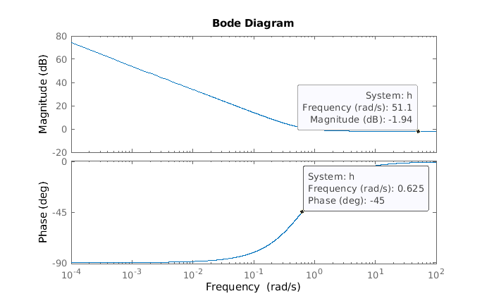
The result is the next.
>> wc = ki/kp

wc =

    0.6250

>> A = 20*log10(kp)

A =

   -1.9382
We can see how the bode diagram matches with the calculated values. Remember that the natural frequency will be 3 dB below the pass-band gain. In this case, since the filter is inverted, we will find the natural frequency 3 dB above the band-pass gain.

The PI regulator can also be expressed with the following equation.
\[H(s)=K_p \left( 1+K_i \cdot \frac{1}{s} \right)\]In this case, the proportional constant multiply both the error and the integral gain. In this case, again, operating a bit we will arrive to a first order high-pass filter.
\[H(s)=K_p \left( \frac{s/K_i+1}{s/K_i}\right)\]Unlike the first implementation, this time the natural frequency of the filter is directly the Ki constant.
\[\omega n = K_i\]This implementation is useful in some cases, but in cases where the system has a lot of gain, for example in some power electronic converters, even a small proportional gain in the regulator can make the system unstable. With the first implementation, we can configure even a 0 in the Kp, but in this second implementation, a 0 in the proportional gain will mean a 0 in the KI, so the regulator won’t work. We will see this in the last example.
PI regulators are widely used in many fields, but in cases where we need a small proportional gain, the regulator will filter at high frequency. This means that, in case of a big and fast disturbance in the plant, the PI regulator will filter it, and it won’t respond. If we want to make the regulator respond to these disturbances, we need to increase the gain in the high-frequency components. This is exactly what we can get by adding a derivative term. In this case, we will talk about the Proportional-Integral-Derivative regulator or PID.
As I mentioned before, the PID regulator includes a derivative term in the equation.
\[H(s) = K_p+K_i\cdot \frac{1}{s}+K_d\cdot s\]Again, let’s operate a bit to isolate the Kp.
\[H(s) = K_p \left(1+\frac{K_i}{K_p}\cdot \frac{1}{s}+\frac{K_d}{K_p}\cdot s \right)\] \[H(s) = K_p \left(\frac{s+\frac{K_i}{K_p}+\frac{K_d}{K_p}\cdot s^2}{s} \right)\]We can see that this time we have a second-order system. In this kind of systems we need to isolate the term \(s^2\).
\[H(s) = K_p \left(\frac{s\frac{K_p}{K_d}+\frac{K_i}{K_d}+ s^2}{s\frac{K_p}{K_d}} \right)\]Once we have this equation, we can see that it is similar to an inverted second-order band-pass filter.
\[H_{BPF}(s)=\frac{\frac{\omega_n}{Q}s}{s^2+\frac{\omega_n}{Q}s+\omega_n^2}\]As we did with the high-pass filter, we can extract for the equations the natural frequency, and in this case, also the quality factor (Q).
\[\omega_n=\sqrt{\frac{K_i}{K_d}}\] \[Q=\frac{K_p}{K_d}\cdot \omega_n\]The gain in the passing band of the filter is configured with the proportional constant. On MATLAB we can check this behavior with the next script.
close all
clear all
clc

s = tf('s');

kp = 0.8;
ki = 0.5;
kd = 0.2;

h = kp+ki/s+kd*s;

w = linspace(0.01,100,300000);
bode(h, w)

w0 = sqrt(ki/kd)
Q = kp/kd*w0
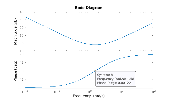
Obtaining the values of the natural frequency and the quality factor we can check its values.
>> w0 = sqrt(ki/kd)

w0 =

    1.5811

>> Q = kp/kd*w0

Q =

    6.3246
Finally, the bode diagram of the PID regulator.

In this article we implemented a PI regulator. Here you can find a small implementation of the same regulator, this time with just one width for the internal and the inputs and outputs. Be careful with this implementation, because it is too simple, and it does not have an anti-windup protection.
module pi #(
  parameter data_width = 32,
  parameter data_width_decimal = 24
)(
  input wire aclk,
  input wire resetn,
  input wire ce,

  input wire signed [data_width-1:0] in, /* Plant output */
  input wire signed [data_width-1:0] reference, /* reference */
  input wire signed [data_width-1:0] kp, /* Proportional constant */
  input wire signed [data_width-1:0] ki, /* Integral constant */
  input wire signed [data_width-1:0] max, /* Maximum output */
  input wire signed [data_width-1:0] min, /* Minimum output */

  output wire signed [data_width-1:0] out /* contro output */
);

  reg signed [data_width-1:0] error;
  wire signed [(data_width*2)-1:0] kp_error; /*  kp error product */
  wire signed [data_width-1:0] kp_error_resized; /* kp error product resized */

  wire signed [(data_width*2)-1:0] ki_error; /* ki error product */
  wire signed [data_width-1:0] ki_error_resized; /* ki error product resized */
  reg signed [data_width-1:0] ki_error_acc; /* Integral accumulator */

  wire signed [data_width-1:0] out_nsat; /* control output before saturation */

  /* error calculation */
  always @(posedge aclk)
    if (!resetn)
      error <= {data_width{1'b0}};
    else
      if (ce)
        error = reference-in;

  /* proportional action */
  assign kp_error = kp * error;
  assign kp_error_resized = $signed(kp_error >>> data_width_decimal);

  /* integral action */
  assign ki_error = ki * error;
  assign ki_error_resized = $signed(ki_error >>> data_width_decimal);

  always @(posedge aclk)
    if (!resetn)
      ki_error_acc <= {data_width{1'b0}};
    else
      if (ce)
        ki_error_acc <= ki_error_resized + ki_error_acc;

  assign out_nsat = kp_error_resized + ki_error_acc;
  assign out = (out_nsat > max)? max:((out_nsat < min)? min:out_nsat);

endmodule
To test this implementation, I use it to control a Buck-Boost converter model. This kind of converter, and all the elevator converters have a lot of gain, so this is one of the cases where even an small proportional gain will make the system unstable. The values for the constants are the next.
kp = 0;
ki = 10*ts;
Notice that the integral gain must be multiplied by the sampling period to match with the continuous system. The test I executed sets a reference of -150 volts (remember that this converter inverts the voltage in its input), and then, at 200 ms the reference is changed to -300 V. The model is runing using a fixed point implementation with 32 bits, and 20 bits in the fractional part.

We can see here the detail of the different magnitudes of the converter.

PI regulators are widely used in the industrial field because you don’t even need to know the model of the plant, or the position of the poles and the zeros of the system. You can make the PI regulator work just by changing the value of the constants until the response of the system is desired. However, knowing the maths of the PI regulator, its bode diagram, and why it works as it works is essential to save time in the regulator adjustment, and also understand why the regulator is not working in some cases. The implementation I showed in this article is not complete, and it can be used as a base for another regulator, but it will work in many different cases. If you want a complete implementation you can check this article, where I implemented a regulator with AXI4 Stream interface and anti-windup. If you are looking for information on complex, or custom regulators, send me an email.


